
                                       1
                     H(z) = -----------------------
                                                 2
                                  r cos(ang)    r
                            1 - 2 ---------- + ----
                                      z          2
                                                z
with r = 0.97 and ang = 2*pi/3. Multiply top and bottom by z^2 to get:
                                       2
                                      z
                     H(z) = -----------------------
                                                 2
                                  r cos(ang)    r
                            1 - 2 ---------- + ----
                                      z          2
                                                z
What are the poles and zeros of this H(z)?
EDU>> Hz = sym('1/( 1 - 2*r*cos(ang)*z^(-1) + r^2*z^(-2))')

Hz =

1/( 1 - 2*r*cos(ang)*z^(-1) + r^2*z^(-2) )

EDU>>pretty(Hz)
EDU>>numerator = [1 0 0]
numerator =
     1     0     0
EDU>>roots(numerator)
ans =
     0
     0
So the zeros are both at z = 0.
Now check for the poles by rooting the denominator polynomial:
EDU>>r = 0.97;
EDU>>ang = 2*pi/3;
EDU>>denominator = [1 -2*r*cos(ang) r^2]
denominator =
     1.0000     0.9700     0.9409
EDU>>roots(denominator)
ans =
  -0.4850 + 0.8400i
  -0.4850 - 0.8400i
EDU>>zprint(ans)
 Z =     X    +     jY     Magnitude    Phase    Ph/pi   Ph(deg)
      -0.485        0.84        0.97    2.094    0.667   120.00
      -0.485       -0.84        0.97   -2.094   -0.667  -120.00

EDU>>zplane(numerator, denominator);
EDU>>axis([xmin xmax ymin ymax]);
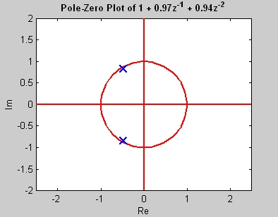
Figure 1. Pole-Zero plot of H(z) = 1/(1 + 0.97z-1 + 0.9409z-2)
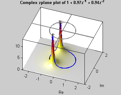
Figure 2. 3D surface plot of H(z) = 1/(1 + 0.97z-1 + 0.9409z-2)
Are the poles and zeros where they should be, based on factoring the polynomials?
Figure 2 is a 3D plot of H(z) over the entire complex Z-plane. You can see the two peaks caused by the poles and the valley in between formed by the zeros at z = 0. The frequency response is is found by evaluating H(z) along the contour defined by z equal ejw. In Figure 1, the unit circle is given for reference; the two poles lie just inside the unit circle. Figure 2 shows a blue line that traces out the unit circle.
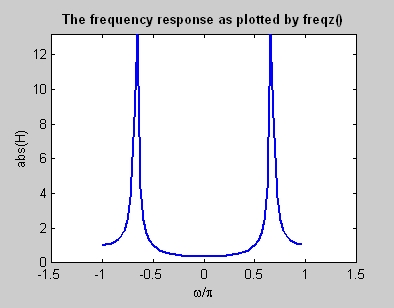
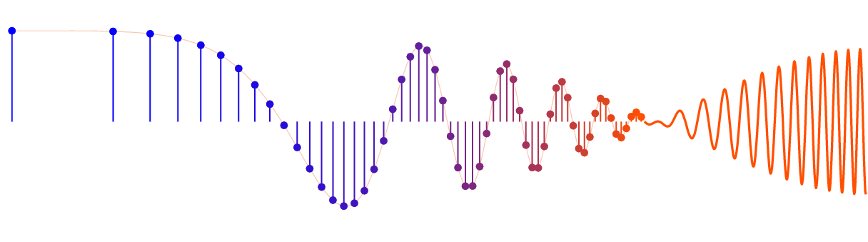
Figure 4 is a movie showing how the frequency response is found by tracing
around the unit circle.
Figure 4. Movie
Here is another movie to help you visualize what is happening
 McClellan, Schafer, and Yoder, Signal Processing First, ISBN 0-13-065562-7.