IIR Filtering Demo

The class of infinite-length impulse response (IIR) filters can be characterized in the three domains: the time domain via the impulse response h[n], the frequency domain via the frequency response, and the z-domain via poles and zeros. This demo shows plots in the three domains for a variety of choices of the feedback coefficients in first- and second-order IIR filters. Similar plots can be generated interactively by using the MATLAB graphical user interface tool called PeZ.

First-Order IIR Filters

Earlier we learned that first-order IIR filters (also called feedback filters) of the form:

y[n] = a y[n-1] + x[n]

have an impluse response given by:

y[n] = aⁿ for n≥0

Usually the parameter a is taken to be a real number. However, if a is chosen to be complex, then the impulse response of the first-order IIR filter can be written as:

y[n] = aⁿ = (r e^jθ) ⁿ = rⁿe^jθn for n≥0

Thus, an oscillating signal (sinusoid) can be produced by specifying the appropriate value for a and taking either the real or imaginary part of the impulse response.

Examples

In the first example let's set the feedback coefficient a to be: a = 1e^jπ/4

In MATLAB we can generate the output using the filter command. Here are the series of MATLAB commands that will generate the first order oscillator:


 >>imp=([0:33]==0);                     % <-- length 34 impulse
 >>y=filter(1,[1 -exp(j*2*pi/8)],imp);  % <-- filter the impulse
 >>plot(real(y))                        % <-- take the real part

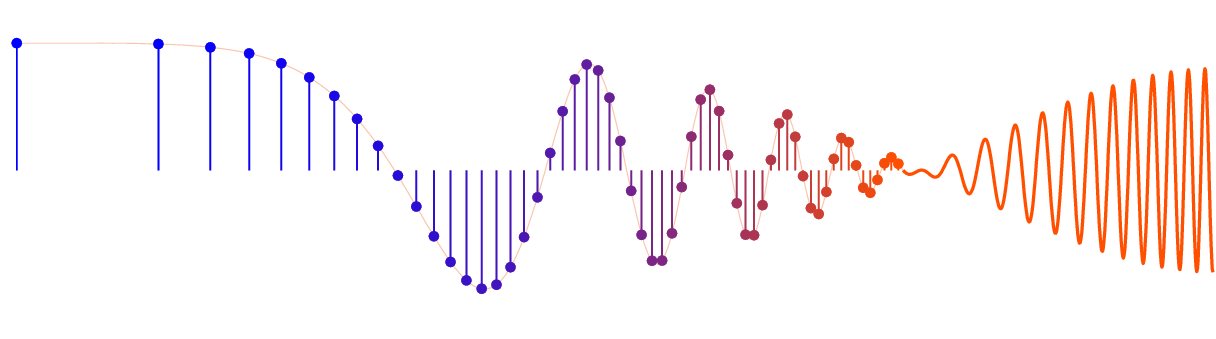
Below is the resultant plot. Note that the "period" of the sinusoid is 8 samples and the digital frequency is therefore 2π/8.

Let's try another example. This time we'll use a = 1 e^jπ/10


 >>imp=([0:40]==0);                      % <-- length 41 impulse
 >>y=filter(1,[1 -exp(j*2*pi/20)],imp);  % <-- filter the impulse
 >>plot(real(y))                         % <-- take the real part

Below is the resultant plot.

This time the frequency of the oscillator is 2π/20. Clearly the angle of the feedback term is equal to the frequency of oscillation.

Second-Order IIR Filters

We also learned about second-order IIR (feedback) filters. Assuming that the poles of the IIR filter are complex, we know that the impulse response will have the following form:

h[n] = Arⁿ cos(nθ + φ).

Assuming the filter coefficients to be strictly real implies that the poles of the filter will occur in conjugate pairs:

p₁ = re^jθ and p₂ = re^-jθ

Expanding the factored polynomial shows the relationship between the filter coefficients, a₁ and a₂, and the magnitude and phase of the poles:

a₁ = 2r cos θ
a₂ = -r²

Remember, the above relationship holds only when the poles are conjugate pairs. By setting a₂ = -1 we can ensure that the oscillator does not decay with time. Now by simply varying a₁ we can control the frequency of oscillation. Below are some examples that demonstrate the relationship between filter coefficients, pole locations and frequency of oscillation.

Example: a₂ Fixed, Variable a₁

In these examples, we will fix a₂ = -1 and observe the oscillator output and pole/zero plot as a₁ is varied from 2 cos(π/6) to 2 cos(π/3).
a₁ = 2 cos(π/6) and a₂ = -1

a₁ = 2 cos(π/4) and a₂ = -1

a₁ = 2 cos(π/3) and a₂ = -1

Note how the magnitude of the poles remains equal to one but the angle changes with a₁. Also note how the amplitude of the oscillator changes for different a₁. This is because a₁ and a₂ do not provide independent control over the amplitude and frequency of the ocsillator.

Example: a₁ Fixed, Variable a₂

In these examples we will fix a₁=2 cos(π/4) and observe the oscillator output and pole/zero plot as a₂ is varied from -0.8 to -1.2.
a₁ = 2 cos(π/4) and a₂ = -0.8

a₁ = 2 cos(π/4) and a₂ = -1

a₁ = 2 cos(π/4) and a₂ = -1.2

Note that as a₂ is changed the the poles move along a vertical line that intersects the x-axis at x = cos(π/4) The filter coefficient a₂ can also be seen to affect the frequency of oscillation. This is because a₁ and a₂ do not provide independent control over the amplitude and frequency of the ocsillator. Note also that if a₂ has magnitude less than one the oscillator decays while if the magnitude of a₁ is greater than one the oscillator grows over time.

Below are a few examples using the MATLAB tool PeZ.

Example: Second Order Oscillator

Using PeZ in MATLAB we can easily generate complex pole pairs. For an oscillator that does not decay we must be careful to place the poles on the unit circle. We will use the edit by coordinate feature of PeZ to insure proper pole placement:

Note the poles have magnitude equal to one and angles equal to π/8. Pez returns the following for plots for the impulse and frequency response:

While it is difficult to measure the frequency of the oscillator from the above graph it can be seen to be approximately 2π/16, which is the value we expected.

Example: Decaying Oscillator

By choosing r < 1, we can generate a sinusoid that decays over time. As an illustration, lets start with previous example and observe how the impulse reponse is affected by decreasing the magnitude r from from 1 to 0.925 (the angle is held fixed at π/8:

Here are the plots for r=1:

Now here are the plots for r=0.975:

Now here are the plots for r=0.95:

Now here are the plots for r=0.925:

Note how the amplitude of the impulse reponse decays faster with smaller values of r.

Example: Growing Oscillator

By choosing r > 1, we can generate a sinusoid that grows over time. As an illustration, lets start with previous example and observe how the impulse reponse is affected by increasing the magnitude r from from 1 to 1.075:

Here are the plots for r=1:

Now here are the plots for r=1.025:

Now here are the plots for r=1.05:

Now here are the plots for r=1.075: